5  LIME Interpretability Evaluation for BERT

5.1 Objective

Systematically evaluate the interpretability of a fine-tuned BERT sentiment model using LIME on all validation tweets: - Extract and aggregate top words by importance - Visualize most influential words via word cloud - Assess explanation consistency under perturbations.

5.2 Background: BERT and the Need for Interpretability

• BERT (Bidirectional Encoder Representations from Transformers) is a deep pre-trained language model capable of understanding contextual relationships in text. It is fine-tuned on downstream tasks such as sentiment classification to achieve state-of-the-art performance.
• However, due to its complexity and non-linearity, BERT behaves like a “black-box” model, making it difficult to understand its predictions.
• LIME helps address this by approximating the local decision boundary around a specific input, allowing us to identify which words influenced the model’s prediction the most.

5.3 Load Model, Tokenizer, and Validation Set

Load the fine-tuned BERT model and tokenizer, and prepare a cleaned sample of tweets from the validation set for explanation.

import torch
from transformers import AutoTokenizer, AutoModelForSequenceClassification
import pandas as pd
import numpy as np
import os

# Disable tokenizer warnings
os.environ["TOKENIZERS_PARALLELISM"] = "false"

# Load model and tokenizer
model_path = "./scripts/bert_model4"
model = AutoModelForSequenceClassification.from_pretrained(model_path)
model.to("cuda")
tokenizer = AutoTokenizer.from_pretrained(model_path)
model.eval()

# Load validation data
class_names = ["Positive", "Neutral", "Negative", "Irrelevant"]
col_names = ["id", "entity", "sentiment", "tweet"]
val = pd.read_csv("data/twitter_validation.csv", header=None, names=col_names)
val = val.dropna(subset=["tweet"])
val = val[val["tweet"].str.strip().astype(bool)]
val = val[val["sentiment"].isin(class_names)].reset_index(drop=True)
#val = val.sample(5, random_state=42)

print(f"✅ Loaded {len(val)} validation tweets")

✅ Loaded 1000 validation tweets

5.4 Setup LIME Explainer and Prediction Function

Define a wrapper function that returns prediction probabilities (needed by LIME), and initialize the LIME explainer with class names.

from lime.lime_text import LimeTextExplainer

# Define prediction wrapper

def bert_predict_proba(texts):
    inputs = tokenizer(texts, return_tensors="pt", padding=True, truncation=True, max_length=128)
    inputs = {k: v.to(model.device) for k, v in inputs.items()}
    with torch.no_grad():
        outputs = model(**inputs)
    probs = torch.nn.functional.softmax(outputs.logits, dim=-1)
    return probs.cpu().numpy()

# Initialize LIME
explainer = LimeTextExplainer(class_names=class_names)

5.5 Run LIME on Validation Set and Collect Word Importances

Word Importances Run LIME on each tweet to get top influential words and their weights. Store the results for later visualization and analysis.

import emoji
import pandas as pd

def clean_text(text):
    no_emoji = emoji.replace_emoji(text, replace='')
    cleaned = no_emoji.encode("utf-8", "ignore").decode("utf-8", "ignore")
    return cleaned

all_weights = []
print(f"Starting explanation on {len(val)} tweets...")

for idx, row in val.iterrows():
    text = clean_text(str(row["tweet"]))
    true_sentiment = clean_text(str(row["sentiment"]))

    try:
        explanation = explainer.explain_instance(
            text_instance=text,
            classifier_fn=bert_predict_proba,
            num_features=10,
            top_labels=1,
            num_samples=100
        )

        label_idx = explanation.top_labels[0]
        pred_label = class_names[label_idx]
        exp_list = explanation.as_list(label=label_idx)

        if not exp_list:
            print(f"⚠️ No explanation for tweet {idx}: {text[:30]}")
            continue

        for word, weight in exp_list:
            all_weights.append({
                "tweet": text,
                "true_label": true_sentiment,
                "pred_label": clean_text(pred_label),
                "word": clean_text(word),
                "weight": weight
            })

    except Exception as e:
        print(f"❌ Error on tweet {idx}: {e}")
        continue

df_weights = pd.DataFrame(all_weights)
print("✅ All explanations completed.")

Starting explanation on 1000 tweets...
✅ All explanations completed.

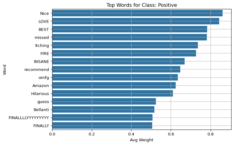
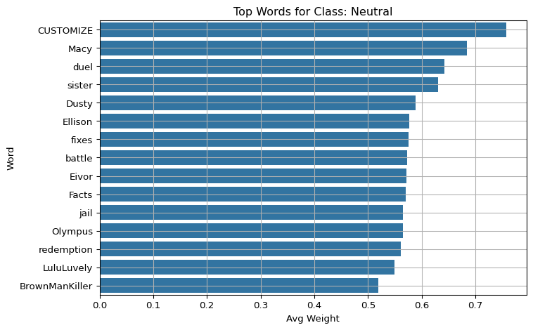
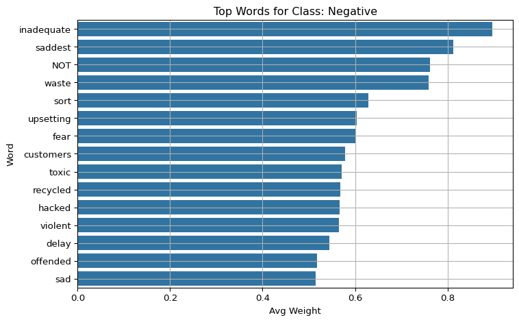
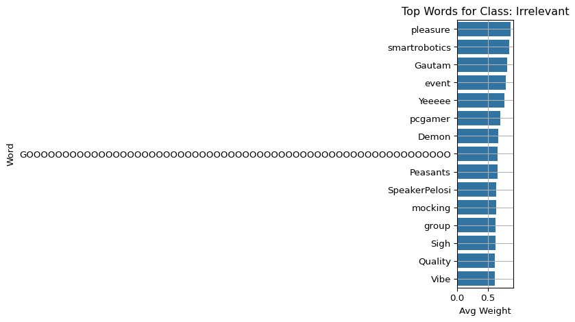
5.6 Visualize Top Words by Class

For each sentiment class, plot the average contribution of the top words that most influenced the model’s predictions for that class.

import matplotlib.pyplot as plt
import seaborn as sns

for label in class_names:
    subset = df_weights[df_weights["pred_label"] == label]
    top_words = subset.groupby("word")["weight"].mean().sort_values(ascending=False).head(15)

    plt.figure(figsize=(8, 5))
    sns.barplot(y=top_words.index, x=top_words.values)
    plt.title(f"Top Words for Class: {label}")
    plt.xlabel("Avg Weight")
    plt.ylabel("Word")
    plt.grid(True)
    plt.tight_layout()
    plt.show()

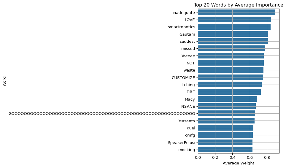
5.7 Visualize Top Words (Mean Weight)

import matplotlib.pyplot as plt
import seaborn as sns

# Top contributing words
top_words = df_weights.groupby("word")["weight"].mean().sort_values(ascending=False).head(20)

plt.figure(figsize=(10,6))
sns.barplot(y=top_words.index, x=top_words.values)
plt.title("Top 20 Words by Average Importance")
plt.xlabel("Average Weight")
plt.ylabel("Word")
plt.grid(True)
plt.tight_layout()
plt.show()

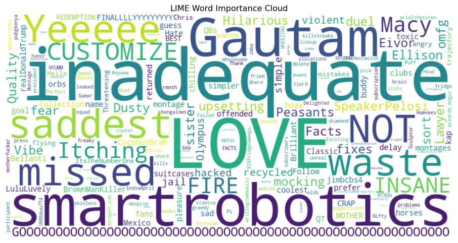
5.8 Word Cloud of Influential Words

Visualize important words using a word cloud, where larger font size indicates higher average contribution to predictions. This is useful for presentations and high-level understanding.

from wordcloud import WordCloud

word_freq = df_weights.groupby("word")["weight"].mean().to_dict()
wordcloud = WordCloud(width=800, height=400, background_color="white").generate_from_frequencies(word_freq)

plt.figure(figsize=(12, 6))
plt.imshow(wordcloud, interpolation="bilinear")
plt.axis("off")
plt.title("LIME Word Importance Cloud")
plt.show()

5.9 Stability Evaluation with Minor Perturbations

Slightly change each tweet by replacing some words with synonyms. Then compare the original and modified LIME explanations using Jaccard similarity to assess explanation stability.

from nltk.corpus import wordnet
import random
import nltk
nltk.download('wordnet')

# Simple synonym substitution for robustness testing
def synonym_replace(text):
    words = text.split()
    new_words = []
    for word in words:
        syns = wordnet.synsets(word)
        if syns and random.random() < 0.2:
            lemmas = syns[0].lemma_names()
            if lemmas:
                new_words.append(lemmas[0].replace("_", " "))
                continue
        new_words.append(word)
    return " ".join(new_words)

# Compare explanations between original and perturbed text
similarities = []

for i in range(len(val)):
    text = val.iloc[i]["tweet"]
    perturbed = synonym_replace(text)

    expl_orig = explainer.explain_instance(
        text,
        bert_predict_proba,
        num_features=10,
        top_labels=1,
        num_samples=100
    )

    expl_pert = explainer.explain_instance(
        perturbed,
        bert_predict_proba,
        num_features=10,
        top_labels=1,
        num_samples=100
    )

    words_orig = set(w for w, _ in expl_orig.as_list(label=expl_orig.top_labels[0]))
    words_pert = set(w for w, _ in expl_pert.as_list(label=expl_pert.top_labels[0]))

    jaccard = len(words_orig & words_pert) / len(words_orig | words_pert)
    similarities.append(jaccard)

print(f"Average Jaccard similarity over {len(val)} samples: {np.mean(similarities):.3f}")

[nltk_data] Downloading package wordnet to
[nltk_data]     C:\Users\16925\AppData\Roaming\nltk_data...
[nltk_data]   Package wordnet is already up-to-date!

Average Jaccard similarity over 1000 samples: 0.465

5.10 Summary

In summary, this section used LIME to interpret a fine-tuned BERT model on tweets, visualized top features, and tested explanation robustness under perturbations (Jaccard: 0.475).