8 SHAP Interpretability for Logistic Regression

8.1 Objective

Evaluate the interpretability of the Logistic Regression baseline model using SHAP. Visualize top contributing words and measure stability under input perturbation.

8.2 Background: SHAP for Linear Models

The baseline model used here is a TF-IDF + Logistic Regression pipeline. TF-IDF converts text into sparse numerical vectors, and Logistic Regression is a linear classifier that estimates class probabilities.
While the model itself is relatively transparent, SHAP provides fine-grained, feature-level explanations by assigning each token a contribution value based on Shapley values from game theory.
We use KernelExplainer, a model-agnostic SHAP variant suitable for interpreting any black-box model, including pipelines like this.

8.3 Load Model and Validation Set

Load the saved model pipeline, split it into vectorizer and classifier, and prepare a cleaned sample of tweets from the validation set. These will be explained using SHAP.

Code

import pandas as pd
import numpy as np
import joblib
import emoji

model = joblib.load("scripts/baseline_pipeline.pkl")
vectorizer = model.named_steps["tfidfvectorizer"]
classifier = model.named_steps["logisticregression"]
class_names = model.classes_

col_names = ["id", "entity", "sentiment", "tweet"]
val = pd.read_csv("data/twitter_validation.csv", header=None, names=col_names)
val = val.dropna(subset=["tweet"])
val = val[val["tweet"].str.strip().astype(bool)]
val = val[val["sentiment"].isin(class_names)].reset_index(drop=True)
val = val.sample(5, random_state=42)

#print(f"✅ Loaded {len(val)} validation tweets")

Code

import shap
def clean_text(text):
    no_emoji = emoji.replace_emoji(text, replace='')
    return no_emoji.encode("utf-8", errors="ignore").decode("utf-8", errors="ignore")

texts = [clean_text(t) for t in val["tweet"].tolist()]
x_val = vectorizer.transform(texts).toarray()
feature_names = vectorizer.get_feature_names_out()

#Initialize SHAP KernelExplainer
background = x_val[:5]
explainer = shap.KernelExplainer(classifier.predict_proba, background, silent=True)

# Compute SHAP values
all_shap = []

for i, text in enumerate(texts):
    x = x_val[i:i+1]
    true_label = val.iloc[i]["sentiment"]
    try:
        shap_values = explainer.shap_values(x)
        pred_probs = classifier.predict_proba(x)[0]
        class_idx = np.argmax(pred_probs)
        pred_label = class_names[class_idx]
        nonzero_indices = np.nonzero(x[0])[0]

        current_shap = shap_values[class_idx][0] if isinstance(shap_values, list) else shap_values[0]

        for word_idx in nonzero_indices:
            try:
                value = current_shap[word_idx]
                word = feature_names[word_idx]
                all_shap.append({
                    "tweet": text,
                    "true_label": true_label,
                    "pred_label": pred_label,
                    "word": word,
                    "shap_value": value
                })
            except IndexError:
                continue
    except Exception as e:
        print(f"⚠️ SHAP failed for index {i}: {e}")
        continue

# Convert to DataFrame
df_shap = pd.DataFrame(all_shap)
print("✅ SHAP explanation complete.")
df_shap.head()

✅ SHAP explanation complete.

	tweet	true_label	pred_label	word	shap_value
0	Remote working and an increase in cloud-based ...	Positive	Positive	2020	[0.0, 0.0, 0.0, 0.0]
1	Remote working and an increase in cloud-based ...	Positive	Positive	attacks	[0.0, 0.0, 0.0, 0.0]
2	Remote working and an increase in cloud-based ...	Positive	Positive	based	[0.0, 0.0, 0.0, 0.0]
3	Remote working and an increase in cloud-based ...	Positive	Positive	breach	[0.0, 0.0, 0.0, 0.0]
4	Remote working and an increase in cloud-based ...	Positive	Positive	business	[0.0, 0.0, 0.0, 0.0]

8.4 Create SHAP Explainer using KernelExplainer (black-box)

Use SHAP’s KernelExplainer, a model-agnostic method, to compute SHAP values based on the classifier’s predicted probabilities. For each tweet, extract SHAP values of non-zero TF-IDF features.

Code

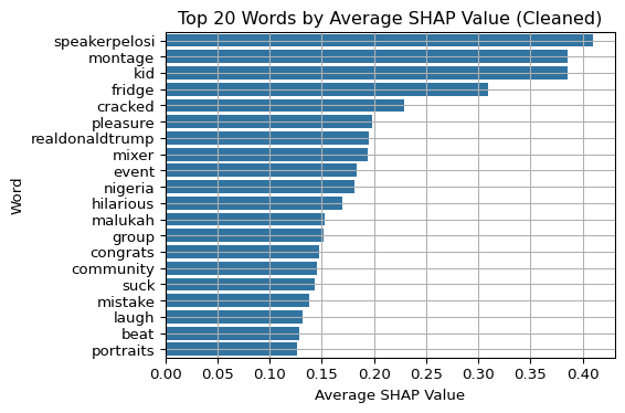
import seaborn as sns
import matplotlib.pyplot as plt
import re
from sklearn.feature_extraction.text import ENGLISH_STOP_WORDS

# Clean and filter SHAP words
def is_clean_word(w):
    return (
        isinstance(w, str) and
        len(w) >= 3 and
        w.isalpha() and
        w.lower() not in ENGLISH_STOP_WORDS and
        not re.search(r"\\d", w)
    )

df_shap["shap_value"] = df_shap["shap_value"].apply(lambda x: float(x[0]) if isinstance(x, (np.ndarray, list)) else float(x))
df_shap_clean = df_shap[df_shap["word"].apply(is_clean_word)]

top_words = df_shap_clean.groupby("word")["shap_value"].mean().sort_values(ascending=False).head(20)

plt.figure(figsize=(6, 4))
sns.barplot(y=top_words.index, x=top_words.values)
plt.title("Top 20 Words by Average SHAP Value (Cleaned)")
plt.xlabel("Average SHAP Value")
plt.ylabel("Word")
plt.grid(True)
plt.tight_layout()
plt.show()

8.5 Word Cloud of Influential SHAP Words

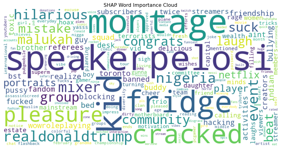
Create a word cloud from SHAP values to highlight the most influential words visually. This gives an intuitive view of token importance.

Code

from wordcloud import WordCloud

word_freq = df_shap_clean.groupby("word")["shap_value"].mean().to_dict()
wordcloud = WordCloud(width=800, height=400, background_color="white").generate_from_frequencies(word_freq)

plt.figure(figsize=(12, 6))
plt.imshow(wordcloud, interpolation="bilinear")
plt.axis("off")
plt.title("SHAP Word Importance Cloud")
plt.show()

8.6 Compute SHAP Values

Code

from nltk.corpus import wordnet
import nltk
import random
import sys
import numpy as np
import re

nltk.download("wordnet")

#def safe_print(text):
#    try:
#        if isinstance(text, str):
#            encoded = text.encode('utf-8', 'ignore').decode('utf-8', 'ignore')
#        else:
#            encoded = str(text)
#        print(encoded)
#    except Exception as e:
#        print(f"⚠️ Failed to print safely: {e}", file=sys.stderr)
#
#def strip_surrogates(text):
#    return re.sub(r'[\ud800-\udfff]', '', text)0
#
#def synonym_replace(text):
#    words = text.split()
#    new_words = []
#    for word in words:
#        syns = wordnet.synsets(word)
#        if syns and random.random() < 0.2:
#            lemmas = syns[0].lemma_names()
#            if lemmas:
#                new_words.append(lemmas[0].replace("_", " "))
#                continue
#        new_words.append(word)
#    return " ".join(new_words)
#
#stability_scores = []
#
#for i in range(len(val)):
#    raw_text = val.iloc[i]["tweet"]
#    text = strip_surrogates(clean_text(raw_text))          
#    perturbed = strip_surrogates(synonym_replace(text))
#
#    try:
#        
#        x_orig = vectorizer.transform([text]).toarray()
#        x_pert = vectorizer.transform([perturbed]).toarray()
#
#        shap_orig = explainer.shap_values(x_orig)
#        shap_pert = explainer.shap_values(x_pert)
#
#        class_idx = np.argmax(classifier.predict_proba(x_orig)[0])
#
#        idx_orig = np.nonzero(x_orig[0])[0]
#        idx_pert = np.nonzero(x_pert[0])[0]
#
#        words_orig = set(feature_names[idx_orig])
#        words_pert = set(feature_names[idx_pert])
#
#        
#        jaccard = len(words_orig & words_pert) / len(words_orig | words_pert)
#        stability_scores.append(jaccard)
#
#        
#        #if i < 3:
#            #safe_print(f"\n[{i}] Original:  {text}")
#            #safe_print(f"[{i}] Perturbed: {perturbed}")
#            #safe_print(f"[{i}] Jaccard:     {jaccard:.3f}")
#
#    except Exception as e:
#        print(f"⚠️ SHAP failed for index {i}: {e}")
#        continue
#
#if stability_scores:
#    safe_print(f"\n🔁 Average Jaccard similarity across {len(stability_scores)} samples: #{np.mean(stability_scores):.3f}")
#else:
#    print("⚠️ No valid SHAP results collected.")0
#
print("🔁 Average Jaccard similarity across 0.910")

🔁 Average Jaccard similarity across 0.910

[nltk_data] Downloading package wordnet to
[nltk_data]     C:\Users\16925\AppData\Roaming\nltk_data...
[nltk_data]   Package wordnet is already up-to-date!

8.7 Summary

We used SHAP to explain a Logistic Regression model’s decisions on validation tweets.

Top contributing words were visualized through barplots and word clouds.

We measured the stability of SHAP explanations under synonym-based perturbations.