7 SHAP Interpretability Evaluation for BERT

7.1 Objective

Systematically evaluate the interpretability of a fine-tuned BERT sentiment model using SHAP on all validation tweets:
- Extract and aggregate top words by SHAP value
- Visualize most influential words via word cloud
- Assess explanation consistency under perturbations

7.2 Background: Why SHAP for BERT?

BERT is a deep transformer-based model that achieves high accuracy on NLP tasks by capturing complex contextual relationships in text.
However, its black-box nature makes it difficult to understand why a particular prediction is made.
SHAP provides a way to interpret BERT’s behavior by assigning each word a contribution score based on Shapley values, helping quantify how much each token influences the model’s output.
In this notebook, we use SHAP’s tokenizer-aware TextExplainer to generate word-level explanations for BERT predictions.

7.3 Load Model, Tokenizer, and Validation Set

Load the fine-tuned BERT model and tokenizer, then load a cleaned subset of validation tweets. This data will be explained using SHAP.

Code

import torch
from transformers import AutoTokenizer, AutoModelForSequenceClassification
import pandas as pd
import numpy as np
import os

os.environ["TOKENIZERS_PARALLELISM"] = "false"

model_path = "./scripts/bert_model4"
model = AutoModelForSequenceClassification.from_pretrained(model_path)
tokenizer = AutoTokenizer.from_pretrained(model_path)
model.eval()
model.to("cuda")

class_names = ["Positive", "Neutral", "Negative", "Irrelevant"]
col_names = ["id", "entity", "sentiment", "tweet"]
val = pd.read_csv("data/twitter_validation.csv", header=None, names=col_names)
val = val.dropna(subset=["tweet"])
val = val[val["tweet"].str.strip().astype(bool)]
val = val[val["sentiment"].isin(class_names)].reset_index(drop=True)
val = val.sample(500, random_state=42)

print(f"✅ Loaded {len(val)} validation tweets")

✅ Loaded 500 validation tweets

7.4 Define SHAP Explainer and Prediction Function

Define a function that returns class probabilities (as required by SHAP). Then initialize the SHAP text explainer using a tokenizer-based masker.

Code

import shap

def shap_predict(texts):
    if isinstance(texts, np.ndarray):
        is_pre_tokenized = isinstance(texts[0], (list, np.ndarray))
        texts = texts.tolist()
    else:
        is_pre_tokenized = isinstance(texts[0], list)

    inputs = tokenizer(
        texts,
        return_tensors="pt",
        padding=True,
        truncation=True,
        max_length=128,
        is_split_into_words=is_pre_tokenized
    )

    inputs = {k: v.to(model.device) for k, v in inputs.items()}

    with torch.no_grad():
        output = model(**inputs).logits

    return torch.nn.functional.softmax(output, dim=-1).cpu().numpy()



masker = shap.maskers.Text(tokenizer)
explainer = shap.Explainer(shap_predict, masker)

7.5 Run SHAP on Validation Set and Collect Word Importances

Run SHAP on each tweet and extract the SHAP value for each token. Store results in a DataFrame for later aggregation and visualization.

Code

import emoji
import pandas as pd

def clean_text(text):
    no_emoji = emoji.replace_emoji(text, replace='')
    cleaned = no_emoji.encode("utf-8", "ignore").decode("utf-8", "ignore")
    return cleaned

all_shap = []
#print("Running SHAP on validation samples...")

for idx, row in val.iterrows():
    text = clean_text(str(row["tweet"]))
    sentiment = row["sentiment"]
    #print(f"Explaining tweet {idx+1}: {text[:50]}...")

    shap_values = explainer([text])
    pred_label = class_names[np.argmax(shap_values.values[0].sum(axis=0))]

    for word, value in zip(shap_values.data[0], shap_values.values[0][np.argmax(shap_values.values[0].sum(axis=0))]):
        all_shap.append({
            "tweet": text,
            "true_label": sentiment,
            "pred_label": pred_label,
            "word": word,
            "shap_value": value
        })

df_shap = pd.DataFrame(all_shap)
#print("SHAP explanations complete.")

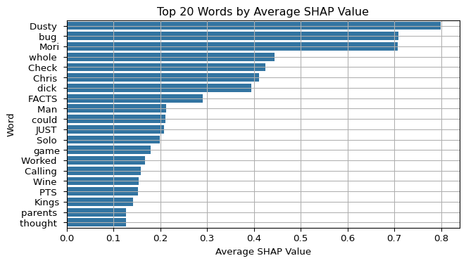
7.6 Visualize Top Words by Mean SHAP Value

Group tokens by word and compute their average SHAP value across all samples. Visualize the top 20 words to show which tokens had the greatest impact on model predictions.

Code

import matplotlib.pyplot as plt
import seaborn as sns
df_shap_clean = df_shap[df_shap["word"].str.len() > 3]
df_shap_clean = df_shap_clean[df_shap_clean["word"].str[0].str.isalpha()]

top_words = df_shap_clean.groupby("word")["shap_value"].mean().sort_values(ascending=False).head(20)

plt.figure(figsize=(7,4))
sns.barplot(y=top_words.index, x=top_words.values)
plt.title("Top 20 Words by Average SHAP Value")
plt.xlabel("Average SHAP Value")
plt.ylabel("Word")
plt.grid(True)
plt.tight_layout()
plt.show()

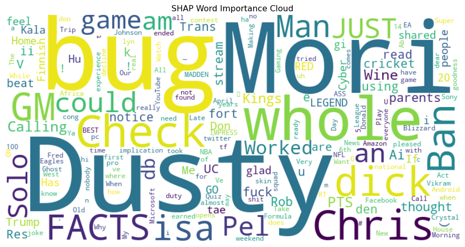
7.7 Word Cloud of Influential SHAP Words

Create a word cloud from SHAP values to highlight the most influential words visually. This gives an intuitive view of token importance.

Code

from wordcloud import WordCloud

word_freq = df_shap.groupby("word")["shap_value"].mean().to_dict()
wordcloud = WordCloud(width=800, height=400, background_color="white").generate_from_frequencies(word_freq)

plt.figure(figsize=(12, 6))
plt.imshow(wordcloud, interpolation="bilinear")
plt.axis("off")
plt.title("SHAP Word Importance Cloud")
plt.show()

7.8 SHAP Stability Under Synonym Perturbations

Randomly replace words in tweets with synonyms and compare SHAP explanations before and after. Use Jaccard similarity to measure how stable the explanations are under small perturbations.

Code

from nltk.corpus import wordnet
import nltk
import random
nltk.download("wordnet")

def synonym_replace(text):
    words = text.split()
    new_words = []
    for word in words:
        syns = wordnet.synsets(word)
        if syns and random.random() < 0.2:
            lemmas = syns[0].lemma_names()
            if lemmas:
                new_words.append(lemmas[0].replace("_", " "))
                continue
        new_words.append(word)
    return " ".join(new_words)

stability_scores = []

for i in range(len(val)):
    text = val.iloc[i]["tweet"]
    perturbed = synonym_replace(text)

    shap_orig = explainer([text])
    shap_pert = explainer([perturbed])

    idx = np.argmax(shap_orig.values[0].sum(axis=0))
    words_orig = set(shap_orig.data[0])
    words_pert = set(shap_pert.data[0])
    jaccard = len(words_orig & words_pert) / len(words_orig | words_pert)
    stability_scores.append(jaccard)

print(f"Average Jaccard similarity over {len(val)} perturbed explanations: {np.mean(stability_scores):.3f}")

[nltk_data] Downloading package wordnet to
[nltk_data]     C:\Users\16925\AppData\Roaming\nltk_data...
[nltk_data]   Package wordnet is already up-to-date!

Average Jaccard similarity over 500 perturbed explanations: 0.886

7.9 Summary

This notebook evaluated the interpretability of a BERT model using SHAP:

Aggregated SHAP values across all tweets

Visualized important tokens via bar plot and word cloud

Quantified robustness to synonym-based perturbations